Turbulent Flow in a Pipe Around an Obstacle (repository)

The Lattice Boltzmann Equation is a versatile model to simulate the dynamics of macroscopic and mesoscopic flows, as it effectively solves the Navier Stokes equation for low Mach numbers. Instead of evolving macroscopic quantities such as the velocity and density profile of the flow, the Lattice Boltzmann Equation evolves the discrete-velocity distribution function $\boldsymbol{f}(\boldsymbol{r}, t)$. Space and time are discretized in this model by taking a number of gridpoints in the domain of interest, and evolving the system stepwise over time. The velocities of the populations are discretized by only taking into account a select few directions. The type of model chosen can be described by the term "DdQn", where 'd' indicates the dimension of the simulation, and 'n' is the number of velocity directions $\boldsymbol{c}_i$ at every gridpoint. For this specific case I used the D2Q9 model [1]. This makes the vector $\boldsymbol{r}$ 2-dimensional, and the distributions $\boldsymbol{f}$ 9-dimensional, containing the populations of each velocity direction. The usual macroscopic quantities can be obtained from $\boldsymbol{f}(\boldsymbol{r}, t)$ in the following manner: \begin{equation} \begin{split} \rho(\boldsymbol{r}, t) &= \sum_i f_i(\boldsymbol{r},t)\\ \boldsymbol{u}(\boldsymbol{r}, t) &= \frac{\sum_i \boldsymbol{c}_i f_i(\boldsymbol{r},t)}{\sum_i f_i(\boldsymbol{r},t)} \end{split} \end{equation} Where $\rho$ is the density and $\boldsymbol{u}$ is the macroscopic velocity. The distributions can now be evolved using the Lattice Boltzmann Equation: \begin{equation} \boldsymbol{f}(\boldsymbol{r} + \boldsymbol{c}_i, t+1) = \boldsymbol{f}(\boldsymbol{r}, t) + \boldsymbol{\Omega} \left[\boldsymbol{f}(\boldsymbol{r}, t) - \boldsymbol{f}^{\text{eq}}(\boldsymbol{r}, t)\right] \end{equation} Where $\boldsymbol{f}^{\text{eq}}(\boldsymbol{r}, t)$ contains the populations if the flow would be in equilibrium. The matrix $\boldsymbol{\Omega}$ is the collision operator, which relaxes the populations $\boldsymbol{f}(\boldsymbol{r}, t)$ toward the equilibrium function. Note that I make use of lattice units from now on, such that the lattice spacing and timestep are given by $\Delta r = \Delta t = 1$. The collision operator that is used in this simulation is the simple BGK operator, given by: \begin{equation} \boldsymbol{\Omega}^{\text{BGK}} = -\frac{1}{\tau} \boldsymbol{I} \end{equation} Where $\boldsymbol{I}$ is the identity matrix and $\tau$ is the relaxation time, which is connected to the kinematic viscosity in the following manner: \begin{equation} \nu = \left(\tau - \frac{1}{2}\right) c_s^2 \end{equation} The equilibrium distributions can be calculated again from the macroscopic quantities: \begin{equation} f_i^{\text{eq}} = w_i \rho(\boldsymbol{r},t) \left(1 + \frac{\boldsymbol{u}(\boldsymbol{r},t) \cdot \boldsymbol{c}_i}{c_s^2} + \frac{(\boldsymbol{u}(\boldsymbol{r},t) \cdot \boldsymbol{c}_i)^2}{2c_s^4} - \frac{|\boldsymbol{u}(\boldsymbol{r},t)|^2}{2c_s^2}\right) \end{equation} Where the parameters $w_i$ are the weights of velocities $\boldsymbol{c_i}$. The speed of sound used in this model is given by $c_s = \frac{1}{\sqrt{3}}$ in lattice units.

$i$	$w_i$	$\boldsymbol{c}_i$
0	$4/9$	$(0, 0)$
1	$1/9$	$(1, 0)$
2	$1/36$	$(1, -1)$
3	$1/9$	$(0, -1)$
4	$1/36$	$(-1, -1)$
5	$1/9$	$(-1, 0)$
6	$1/36$	$(-1, 1)$
7	$1/9$	$(0, 1)$
8	$1/36$	$(1, 1)$

The simulation can now be started by initializing the density and velocity profile of the flow. In this case, the initial density profile is set to unity at every gridpoint, and the starting velocities $\boldsymbol{u}$ are zero. With this, the starting equilibrium populations $\boldsymbol{f}^{\text{eq}}$ can be calculated, and we assume that the starting populations $\boldsymbol{f}$ are in equilibrium. This allows us to start the evolution of $\boldsymbol{f}$.

The Lattice Boltzmann Equation can be split into two parts: the collision step and the streaming step. The collision step is given by: \begin{equation} \boldsymbol{f}^\ast(\boldsymbol{r}, t) = \boldsymbol{f}(\boldsymbol{r}, t) - \frac{1}{\tau} \left(\boldsymbol{f}(\boldsymbol{r}, t) - \boldsymbol{f}^{\text{eq}}(\boldsymbol{r}, t)\right) \end{equation}

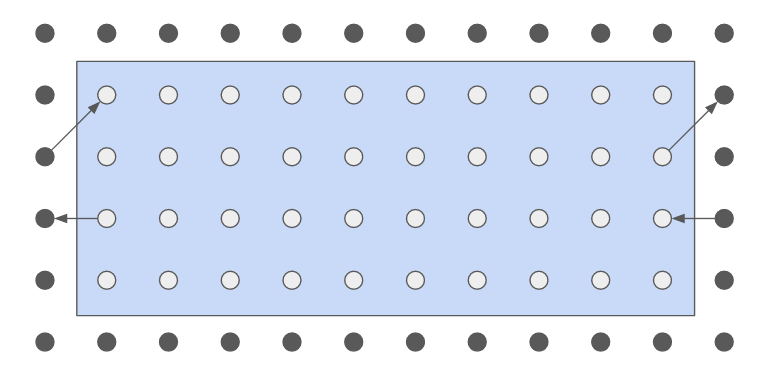
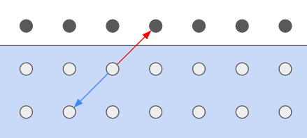
After the collision step, we can perform the streaming step, completing the Lattice Boltzmann Equation: \begin{equation} f_i(\boldsymbol{r}, t + 1) = f_i^\ast(\boldsymbol{r} - \boldsymbol{c}_i, t) \end{equation} Boundary conditions have to be taken into account during the streaming step. This specific simulation makes use of periodic boundary conditions connecting the left and right of the domain. Periodic boundary conditions applied on the distribution function can be written down in a general manner: \begin{equation} \boldsymbol{f}^\ast(\boldsymbol{r} + \boldsymbol{L}, t) = \boldsymbol{f}^\ast(\boldsymbol{r}, t) \end{equation} Where $\boldsymbol{L}$ is a vector containing the sidelengths for a square domain. This means that the populations streaming out of the domain on the right side enter the nodes on the left, and vice versa.

So the streaming equation can be modified as: \begin{equation} f_i(\boldsymbol{r}, t + 1) = f_i^\ast\left(\left(\boldsymbol{r} - \boldsymbol{c}_i\right) \%\, \boldsymbol{L}, t\right) \end{equation} Where the percent sign indicates an element-wise modulo operation. On the top and bottom of the domain I need to implement the solid walls of the pipe. To conserve mass, populations streaming out of the wall should bounce back. Both directions of the velocity of the populations streaming out of the domain are reversed. This brings us to an additional streaming condition if populations stream into a solid wall: \begin{equation} f_i(\boldsymbol{r}, t + 1) = f_j^\ast(\boldsymbol{r}, t) \end{equation} When $\boldsymbol{r} - \boldsymbol{c}_i$ lies on one of the solid nodes inside the wall. The index $j$ is then given by $\boldsymbol{c}_j = -\boldsymbol{c}_i$. This type of boundary condition is called halfway bounce-back, where the populations streaming out of the domain are hit the wall after a time of $\Delta t / 2$ and return back to the same node at $\Delta t$. It is assumed that the actual wall positions $\boldsymbol{r}_w$ are halfway between the outermost fluid nodes, called boundary nodes and denoted by $\boldsymbol{r}_b$, and the solid nodes just inside the wall $\boldsymbol{r}_s$.

A few terms need to be added to the previously stated equations if we want to introduce an external force density $\boldsymbol{F}(\boldsymbol{r}, t)$ on the fluid. When calculating the macroscopic quantities from the distribution function $\boldsymbol{f}$, a term has to be added to the velocities: \begin{equation} \boldsymbol{u}(\boldsymbol{r}, t) = \frac{\left(\sum_i \boldsymbol{c}_i f_i(\boldsymbol{r},t)\right) + \frac{1}{2}\boldsymbol{F}(\boldsymbol{r}, t)}{\sum_i f_i(\boldsymbol{r},t)} \end{equation} Additionally, a source term needs to be added to the collision step: \begin{equation} \boldsymbol{f}^\ast(\boldsymbol{r}, t) = \boldsymbol{f}(\boldsymbol{r}, t) - \frac{1}{\tau} \left(\boldsymbol{f}(\boldsymbol{r}, t) - \boldsymbol{f}^{\text{eq}}(\boldsymbol{r}, t)\right) + \boldsymbol{S}(\boldsymbol{r}, t) \end{equation} With \begin{equation} S_i(\boldsymbol{r}, t) = \left(1 - \frac{1}{2 \tau}\right) w_i \left[\frac{\boldsymbol{c}_i - \boldsymbol{u}(\boldsymbol{r}, t)}{c_s^2} + \frac{\boldsymbol{c}_i \cdot \boldsymbol{u}(\boldsymbol{r}, t)}{c_s^4}\boldsymbol{c}_i\right] \cdot \boldsymbol{F}(\boldsymbol{r}, t) \end{equation} According to the Guo model. The complete algorithm can now be represented in the following way:

References

[1] T. Krueger, H. Kusumaatmaja, A. Kuzmin, O. Shardt, G. Silva, and E. Viggen, The lattice boltzmann method: principles and practice, English, Graduate Texts in Physics (Springer, 2016).