Creating Fractals With the Double Pendulum (repository)

A dynamic fractal can be created by simulating the movement of a double pendulum for many different starting positions.

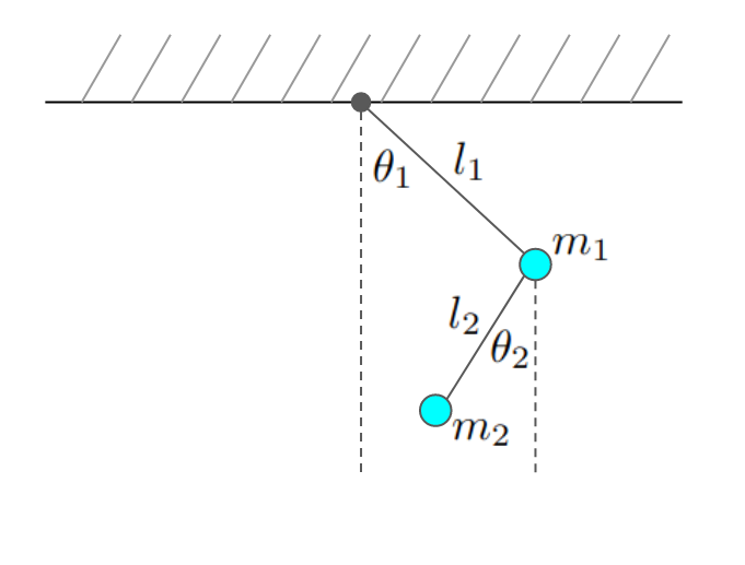
The kinetic and potential energy of this system can be calculated: \begin{equation} \begin{split} &T = \frac{1}{2} m_1 \left(l_1 \dot{\theta_1}\right)^2 + \frac{1}{2}m_2\left[\left(l_1\dot{\theta}_1\right)^2 + \left(l_2\dot{\theta}_2\right)^2 + 2 l_1 l_2 \dot{\theta}_1\dot{\theta}_2 \cos(\theta_1 - \theta_2)\right]\\ &U = -m_1 g \left(l_1 \cos\theta_1\right) - m_2 g \left[l_1 \cos\left(\theta_1\right) + l_2 \cos\left(\theta_2\right)\right] \end{split} \end{equation} Where a dot indicates the time derivative $\frac{d}{dt}$ and $g$ indicates the gravitational acceleration. The potential energy is set to zero at the ceiling. The lagrangian is calculated as: \begin{equation} L = T - U \end{equation} Which brings us to the equations of motion using Lagrange's equations: \begin{equation} \begin{split} &\frac{\partial L}{\partial \theta_1} - \frac{d}{dt}\frac{\partial L}{\partial \dot{\theta_1}} = 0\\ &\frac{\partial L}{\partial \theta_2} - \frac{d}{dt}\frac{\partial L}{\partial \dot{\theta_2}} = 0 \end{split} \end{equation} These equations can be rewritten in the following way: \begin{equation} \begin{split} &\ddot{\theta_1} = -\frac{(2 m_1 + m_2)g\sin(\theta_1) + m_2 g \sin\left(\theta_1 - 2 \theta_2\right) + 2 m_2\sin\left(\theta_1 - \theta_2\right)\left(l_2\dot{\theta_2}^2 + l_1\dot{\theta_1}^2 \cos \left(\theta_1 - \theta_2\right)\right)}{l_1 \left(2 m_1 + m_2 - m_2 \cos \left(2\theta_1 - 2\theta_2\right)\right)}\\ &\ddot{\theta_2} = \frac{2 \sin \left(\theta_1 - \theta_2\right)\left[l_1 (m_1 + m_2) \dot{\theta_1}^2 + (m_1 + m_2) g \cos \left(\theta_1\right) + l_2 m_2 \dot{\theta_2}^2 \cos \left(\theta_1 - \theta_2\right) \right]}{l_1 \left(2 m_1 + m_2 - m_2 \cos \left(2\theta_1 - 2\theta_2\right)\right)} \end{split} \end{equation} Which can be converted to a system of four ordinary differential equations by using $\omega_1 \equiv \dot{\theta_1}$ and $\omega_2 \equiv \dot{\theta_2}$. These equations can now be solved numerically using the Runge-Kutta method.